胡刚 , 宋慧
, 宋慧
HU Gang, SONG Hui
中图分类号: S157/TP306
文献标识码: A
文章编号: 1000-0690(2015)11-1482-07
收稿日期: 2014-06-18
修回日期: 2014-09-19
网络出版日期: 2015-11-20
版权声明: 2015 《地理科学》编辑部 本文是开放获取期刊文献,在以下情况下可以自由使用:学术研究、学术交流、科研教学等,但不允许用于商业目的.
基金资助:
作者简介:
作者简介:胡 刚(1976-),男,山东滨州人,博士,主要从事土壤侵蚀、环境演变、水土资源利用与3S应用研究。E-mail:geo_hug@126.com
展开
摘要
在总结以往LS因子相关算法研究基础上,结合McCool的LS因子参照值,对LS算法的适用性进行评价分析。研究表明,除去复合算法和Remortel修正算法外,其他不同算法LS因子值都小于参照值;研究区LS因子值的最优算法为基于Remortel迭代运算的修正算法;其次为结合刘宝元的陡坡公式和Remortel改进L指数因子迭代运算的复合算法,以及Remortel第4版AML程序算法;再次为Böhner算法,而Moore算法和Desmet算法,由于其与参照值的相关性相对较差,而且其RMSE相对较大,不推荐在该区使用。
关键词:
Abstract
The Universal Soil Loss Equation (USLE) model and its principal derivative and the Revised Universal Soil Loss Equation (RUSLE) model have been widely used in the past decades. However, the use of USLE and RUSLE has been limited by the inability to generate reliable estimates of the LS factor. Several different LS factor algorithms from the previous studies were briefly summarized in this article and their applicability was evaluated in Wohushan reservoir basin. According to the Agriculture Handbook No. 703 and 537 of US Agriculture Department, the LS-values in McCool's table are the same as the LS algorithms in USLE/RUSLE. Although there is some regional heterogeneity in the specific regional applications for LS calculations, the difference is very limited within a certain slope length and slope gradient. Based on these reasons, the LS-values from McCools are primarily preferred as the reference value. There are four basic LS algorithms which were Remortal, Moore, Desmet and Böhner used to be compared with reference value. In addition, two revised algorithms, i.e. the improved iterative Remortal algorithm and complex algorithm, were presented. The slope-length exponent (m) in the former algorithm was revised from low rill/interrill ratio class to moderate class. The complex algorithm was composed of L-factor and S-factor from different research, of which the latter was from the above mentioned improved algorithm of Remortel and S-factor was made up of S algorithm from McCool and that of Liu BY. In this article, the LS values of the six above algorithms were compared with that of McCools by RMSE (the Root Mean Square Error), the correlation coefficient and the slope of the regression equation. The results indicated that, other than the improved algorithm of Remortel and the complex algorithm, the LS-value obtained by different algorithms are all less than that of reference value. It is also found that the optimal algorithm in the study area is the improved iterative algorithm of Remortel, followed by both the AML program of LS factor from RUSLE Version 4 of Remortel and the complex algorithm. The Böhner’s algorithm could also be used in this area. However, the algorithms from Moore and Desmet were recommended not to use in the study area because of their relatively higher RMSEs and relatively poor correlation coefficients.
Keywords:
过去几十年,USLE及其修订版RUSLE被广泛用以估算片蚀和细沟侵蚀的年均土壤流失量。模型中地形对土壤侵蚀的影响,用无量纲的LS因子来计算表示,其中L表示坡长因子,S表示坡度因子。坡长因子L描述了坡长与土壤侵蚀量之间的定量关系,USLE和RUSLE中的L因子表示标准化到22.13 m坡长上的土壤侵蚀量[1]。坡度因子S则反映了坡度对侵蚀的影响[2]。
坡长指坡面漫流的起点到坡度减小至有沉积发生位置的水平距离,或者到径流汇聚的固定渠道的水平距离[3]。坡长的量化有不同的方法和算法,概括来讲,有栅格网格累积法[4]、单位径流能量理论方法[5]、汇水面积法[6]和网络三角技术[7]等。Hickey等较早提出了基于AML(ArcMacro language)的坡长因子算法[8],之后Remortel对其算法进行了改进[9],并基于C++语言开发了坡长因子计算程序,实现了ASCII格式的DEM的读取[10]。国内学者也对此做过相关研究,如罗红等设计出基于AML语言提取坡长值的最大溯源径流路径法[11],张宏鸣等以Remortel的LS算法为基础,设计出利用正向-反向遍历算法取代原累积坡长的算法,运行效率有了较大提高[12]。张宏鸣等提出了适合于流域或区域尺度侵蚀坡长提取与分析的分布式侵蚀坡长提取算法[13]。汪邦稳等[14]对Remortel的程序[9]进行了改进,将产生坡面侵蚀的临界坡度作为确定坡长截止位置的一个限制条件加入到程序中,提高了该程序在黄土高原地区的适用性。尽管如此,自USLE问世以来,坡长因子始终是最具争议的侵蚀影响因子,也是模型应用的主要限制因素[15,16]。
坡度的计算方法也有很多,例如邻域、二次曲面、最大坡度、最大坡降坡度等[10]。不同算法和方法会对坡度结果产生影响,而且误差来源和性质的差异也会导致出现截然不同的结论。如Skidmore[17]、Florinsky[18]认为三阶差分坡度算法精度高于二阶差分算法,而Hodgson[19]、Jones[20]的研究则表明二阶差分算法能给出较三阶差分算法精度高的坡度坡向计算结果。李天文[21]、刘学军[22]等通过对坡度坡向算法的理论分析,结合实验数据得出所有的三阶差分算法中以三阶不带权差分算法精度最高。Hickey等[23]通过不同坡度算法的比较,得出最大坡降坡度保留了原有DEM局地变异,而没有高估坡度。本研究S因子的计算算法采用最大坡降坡度法。
地形因子尽管可以分成坡度因子和坡长因子,而在侵蚀预测应用中,坡度和坡长因子一般一起评价计算[2]。对于LS因子值的计算,由于不同水蚀地区的土壤类型及地形地貌差异,需选择典型样区,计算LS因子值并分析算法的地区适用性[13]。
作为全国水土保持区划方案一级分区的北方土石山区[24],地表土石混杂,石多土少,与其他水土流失严重区域相比,尽管土壤侵蚀量相对有限,但土壤流失后,地面呈现砂砾化或石化,使得土壤农业利用价值大大降低或丧失。鲁中南山地丘陵区是北方土石山区的典型代表,也是该一级分区下面13个3级分区之一。本文选择位于鲁中南山地丘陵区的卧虎山水库流域作为研究对象,在总结各种LS因子值的相关算法基础上,对其区域适用性进行评价分析。
本文所涉及研究区为位于泰山北麓的济南市南部山区卧虎山水库流域,地理位置介于116°56′24″~117°20′24″E、36°19′48″~36°41′24″′N,水库流域面积559 km2。水库流域由锦绣川、锦阳川、锦云川三川流域组成,玉符河即发源于此。卧虎山水库是济南市唯一的一座大型水库,上游串联中型水库一座——锦绣川水库(流域面积166 km2 ),小型水库16座,塘坝42座。水库流域内花岗岩、花岗片麻岩占31 %,石灰岩占69 %。流域土壤类型主要由粗骨土、棕壤、潮土、褐土组成。流域多年平均降水量698 mm,多年平均径流量0.735×10⁸m3。作为城市重要的饮用水水源地,年均供水量2 000×104m3,占全市供水量的3%~5%,年回灌补源用水量3 000×104m3,为济南泉水常年持续喷涌起到了积极作用。
LS因子值算法的适用性是本研究的重点,在总结前人已有LS因子值算法基础上,基于DEM数据计算研究区各种算法的LS因子值。同时,根据McCool等的研究成果[25],得到LS因子参照值,并进行两者的对比分析。本文之所以将McCool之值作为参照值,是因其值及计算方法是根据10 000多个径流小区实测资料归纳整理得到,具有一定的理论普适性,这也是USLE/RUSLE得以广为应用的原因所在。
本研究所用DEM数据为来源于NASA的30 m分辨率ASTER GDEM数据,需要说明的是,该数据在局部水库、湖泊等平坦区域存在异常。为消除误差,通过实地GPS测量,结合部分1∶5万地形图及googleearth遥感影像进行校正。本研究所用图件统一到WGS84坐标系下,使用UTM投影。
在与参照值进行对比分析时,考虑到数据量,在依据不同算法生成的LS因子值流域分布图上,利用HawthsTools工具随机生成200个点,并提取其LS因子值用以对比。地形因子参照标准LS值,采用McCool等研究成果中的数据[25],该表中地形因子LS值适用于细沟侵蚀和细沟间侵蚀比率中等的情形,表中坡度范围为0.2%~60%,坡长范围为0.9~305 m,在表中列出了上述范围中数个标准坡度和标准坡长,以及在标准坡度和坡长下的LS因子值。由于流域实际的坡度和坡长值并非一定是标准坡度和标准坡长值,落入标准坡度坡长区间的LS值,则采用Kriging插值得到。由于选择流域的坡度和坡长值,有部分超出McCool等研究成果的坡度[25](最大到60%)和坡长值(最长到1 000 ft,约合305 m)的范围,因此实际参与对比分析的数据点共有136个(表1)。
表1 流域随机分布136点的坡度及坡长相关参数
Table 1 The related parameters of slope gradient and slope-length for randomly distributed 136 points in Wohushan Reservoir Basin
| 最大值 | 最小值 | 平均值 | 标准偏差 | |
|---|---|---|---|---|
| 坡度(%) | 58.92 | 3.33 | 31.24 | 11.87 |
| 坡长(m) | 293.34 | 15.00 | 137.36 | 75.10 |
在分析时主要用回归分析及均方根误差(the Root Mean Square Error,RMSE,公式中量用RRMSE表示),RMSE计算如下:
其中,
Remortel [9]的AML程序算法的基本过程为,在完成填挖处理的栅格DEM上,计算每个栅格单元的水流来向和去向基础上,从高到低,利用多重循环和迭代方法,完成累计坡长的计算。在该算法中,坡长起点定义为无径流汇入的栅格单元,坡长终点则约定为当下坡单元坡度减少50 %以上发生沉积时即为终点。
目前Remortal的AML程序算法已经发展到第4版,该版程序中坡长指数m的取值较之前版本更为精细,具体为应用McCool等研究成果中的值[26],并通过局部内插得到。而坡度因子则是根据McCool等于1987年提出的S因子公式[27]计算得来。
坡长因素考虑了坡面的纵坡面形态对侵蚀的影响,但没有考虑坡面的平面形态对侵蚀的影响,为了弥补这一缺陷,单位汇水面积(The Unit Contributing Area)得以在坡长因子计算中引入,使其能够体现复杂地形对侵蚀的影响。
Moore等基于单位径流能量理论方法,推导出以单位汇水面积为基础的LS因子算法[28]。该算法中L和S因子作为一个整体来考虑,单位汇水面积体现了径流汇集和分散(即凹型和凸型坡面)的情形,与原有的经验公式相比,更适合复杂地形地貌。
Desmet算法[29]同样以单位汇水面积为基础,但算法中将L和S因子单独考虑,其中L因子的计算中仅考虑栅格入口处的汇水面积,同时加入了以坡度为自变量的修正系数。对于S因子而言,如Desmet所言[29],基于栅格数据的坡度因子计算可以采用不同的方法,本研究中流算法的坡度因子计算采用McCool等人的研究成果[27]。栅格DEM中每一栅格的LS因子值可以通过L和S的乘积得到。
Böhner算法[30]是基于输沙指数(Sediment Transport Index)得到,输沙指数整合集水区的加权平均坡度,以覆盖整个斜坡和局部的过程差异[30],因为水沙的传输过程尤其对于斜坡下部的依赖性更强。
以上述及算法,限于篇幅在此仅作简要介绍,详情可参见相关文献资料。
1) Remortel修正算法。在上述Remortel第4版AML程序算法中,其计算的前提为假设牧场和林地有低侵蚀敏感性,也即意味着在该算法程序中坡长指数(m)取细沟和细沟间侵蚀之比较低情形下的数值,而这和本研究中所依据的LS因子参照值数据适用于细沟侵蚀和细沟间侵蚀比率中等的情形有所不同。这也是之后分析中Remortel算法计算结果小于参照值的原因。
据此我们对Remortel第4版AML程序算法进行了修正,根据McCool等研究成果中的值[25],将坡长指数(m)修改为适用于细沟和细沟间侵蚀之比中等情形下的数值,并将其称为Remortel修正算法。
2) 复合算法。USLE和RUSLE中S因子的设计主要针对缓坡,刘宝元等研究表明,对于坡度大于10°的坡面,应用McCool的坡度因子公式会产生比较大的误差[31],并根据安塞、天水、绥德径流小区的数据得到了陡坡的坡度因子公式。
对于研究区的坡度而言,大于10°的坡面占到总面积的60.61%,因此如果根据McCool的坡度因子公式计算LS因子值,可能会出现较大偏差。为了寻找更适合研究区的LS因子值算法,本研究将McCool的坡度因子算法[27]与刘宝元的陡坡坡度公式[31]相结合,即采用如下的坡度因子计算公式:
坡长因子还是采用的Remortel修改后的迭代运算算法,两者结合得到LS因子值。
在上述LS因子算法设计中,Moore、Desmet及Böhner算法都涉及到汇水面积或单位汇水面积的计算,而这两者又依赖于径流流向算法的设计[31,32]。径流流向算法总体来讲可以分为单流向算法和多流向算法,单流向算法将源栅格的物质流转入下坡的唯一栅格,而多流向算法则会将源栅格的物质流分到多个接收栅格。两者算法的直接结果为,单流向算法会出现平行流和收敛流的情形,而多流向算法则会有分散流的出现[29],而且单流向算法对细小的错误非常敏感[33]。
根据初步研究,在计算LS值过程中涉及到的水流流向算法中,D8算法得到的结果与相关研究结论更为相符,因此在本研究中采用D8流向算式法计算相关参数。
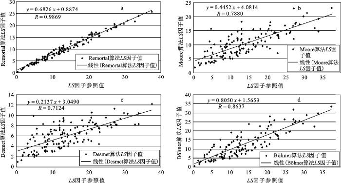
根据随机点提取坡度和坡长,得到相同坡度和坡长条件下的不同算法LS因子值。136个随机点的不同算法LS值与参照值如图1所示。
由图1看出,Remortel算法与参照值的相关性最好,其相关系数达到0.986 9,其次依次为Böhner算法、Moore算法及Desmet算法,相关系数分别为0.863 7、0.788 0和0.712 4。从回归分析得到的线性方程的斜率来看,4种算法的回归方程斜率都小于1,说明与参照值相比,4种算法得到LS因子值都相对偏小,从回归线与1∶1线的关系也可以清楚的看出这一点(图1)。4种算法中,Böhner算法的回归线性方程斜率达到了0.805,是4种算法中最为接近1的,说明根据Böhner算法得到的LS因子值在4种算法中与参照值最为接近,系统误差相对较小。这一点也可以从参照值与各算法LS因子值的均方根误差看出(表2),4种传统算法中Böhner算法的均方根误差为4.18,为传统算法中最小的,其次从小到大依次为Remortel、Moore、Desmet算法。这说明尽管如前所述Remortel算法与参照值的相关性最好,但该算法得到的LS值与参照值的拟合程度还是稍弱于Böhner算法,4种传统方法中Böhner算法与参照值拟合最好。
图1 不同算法LS因子值的计算值与参照值的比较
Fig.1 Comparison of reference value with calculated LS value from different algorithm
表2 不同算法LS因子值的均方根误差
Table 2 RMSE of LS value from different algorithm
| Desmet | Moore | Remortel | Böhner | 修改算法 | 复合算法 | |
|---|---|---|---|---|---|---|
| RMSE | 10.15 | 6.31 | 4.41 | 4.18 | 0.44 | 4.12 |
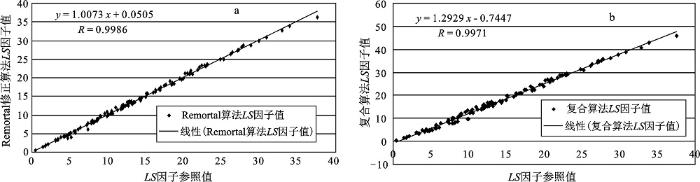
Remortel修正算法计算值与参照值对比如图2a所示,可以看到两者都具有良好的相关性和一致性,两者的相关系数达到了0.998 6,其与参照值的均方根误差也只有0.44,线性回归线也与1∶1线近乎重合。
复合算法计算值与参照值的相关关系如图2b所示。可以看到尽管两者的线性相关系数达到0.997 1,高于 Remortel第4版LS因子算法的相关系数0.986 9,但其均方根误差达到4.12,大于修改后的Remortel算法计算值的RMSE。同时无论从线性方程的斜率,还是线性回归线和1∶1线的关系看,复合算法的计算值大于McCool的LS因子参考值。
通过上面的分析可以看出,对于研究区而言,除去采用刘宝元陡坡S因子和Remortel迭代运算L因子的复合算法及Remortel修正算法计算结果大于参照值外,其他相关算法的计算值都小于McCool的参照值。就计算值与参照值的相关性而言,修改坡长指数(m)的Remortel修正算法和根据刘宝元陡坡公式修正的复合算法相关性最好,两者分别达到了0.998 6和0.997 1,但两者的均方根误差则相差较大,复合算法的RMSE达到了4.12,而Remortel修正算法则只有0.44。其他算法计算值与参照值的相关性从大到小依次为Remortel算法、Böhner算法、Moore算法和Desmet算法,相关系数分别为0.986 9、0.863 7、0.788 0和0.712 4,而就这四种算法的RMSE而言,则分别为4.41、4.18、6.31和10.15。
图2 改进算法LS因子值的计算值与参照值的比较
Fig.2 Comparison of reference value with calculated LS value from combination algorithm
综合相关性和均方根误差两个方面,我们认为研究区LS因子值的最优算法为Remortel修正算法,其次为综合刘宝元陡坡因子和Remortel改进L因子迭代算法的复合算法,再次可以考虑应用Remortel的第4版AML计算程序算法和Böhner算法,而对于Moore算法和Desmet算法而言,由于其与参照值的相关性相对较差,而且其RMSE相对较大,则不推荐在该区使用。
LS因子作为土壤侵蚀模型的重要参数,选择合适的区域LS算法,对于提高土壤侵蚀模型的预报精度具有重要意义。本文通过以上分析初步得出以下结论:
1) 对于研究流域来讲,与参照值相比,根据Remortel、Moore、Desmet及Böhner算法得到的LS因子值都相对偏小。与之相比,根据刘宝元陡坡公式计算得到的S因子与Remortel改进算法迭代得到的L因子相结合的复合算法,计算值比参照值明显要大。
2) 从不同算法得到的LS因子值与参照值的相关性而言,相关性最高的是Remortel改进算法和根据刘宝元陡坡公式改进的复合算法,两者相关系数近乎一致,分别达到了0.998 6和0.997 1,但复合算法的RMSE为4.12,要远大于Remortel改进算法的0.44;其次为Remortel算法和Böhner算法,与参照值的相关系数两者分别为0.986 9和0.863 7,但Remortel算法的RMSE稍大于Böhner算法。与之相比,计算值与参照值相关性较差的为Moore算法和Desmet算法,相关系数分别为0.788 0和0.712 4,RMSE也是几种算法中相对较大的,Desmet算法的RMSE为几种算法中最大的,达到了10.15。
3) 综合考虑计算值与参照值的相关性和均方根误差,研究区LS因子值的最优算法为Remortel修正算法,其次为结合刘宝元的陡坡公式和Remortel改进L因子迭代算法的复合算法,以及Remortel的第4版AML计算程序算法,再次为Böhner算法,而Moore算法和Desmet算法,由于其与参照值的相关性相对较差,而且其RMSE相对较大,不推荐在该区使用。
需要说明的是本研究中仅将各种算法的LS因子计算值与McCool的参照值进行了对比,在实践中还需要进一步检验。
The authors have declared that no competing interests exist.
| [1] |
Shi P J et al.Slope length effects on soil loss for steep slopes [J].https://doi.org/10.2136/sssaj2000.6451759x URL [本文引用: 1] 摘要
ABSTRACT Empirical soil erosion models continue to play an important role in soil conservation planning and environmental evaluations around the world. The effect of hillslope length on soil loss, often termed the slope length factor, is one of the main and most variable components of any empirical model. In the most widely used model, the Universal Soil Loss Equation (USLE), normalized soil loss, L, is expressed as a power function of slope length, lambda, as L = (lambda/22.1)m, in which the slope exponent, m, is 0.2, 0.3, 0.4, and 0.5 for different, increasing slope gradients. In the Revised Universal Soil Loss Equation (RUSLE), the exponent, m, is defined as a continuous function of slope gradient and the expected ratio of rill to interrill erosion. When the slope gradient is 60% and the ratio of rill to interrill erosion is classified as moderate, the exponent m has the value of 0.71 in RUSLE, as compared with 0.5 for the USLE. The purpose of this study was to evaluate the relationship between soil loss and slope length for slopes up to 60% in steepness. Soil loss data from natural runoff plots at three locations on the Loess Plateau in China and data from a previous study were used. The results indicated that the exponent, m, for the relationship between soil loss and the slope length for the combined data from the three stations in the Loess Plateau was 0.44 (r2 = 0.95). For the data as a whole, the exponent did not increase as slope steepness increased from 20 to 60%. We also found that the value of m was greater for intense storms than for less intense storms. These experimental data indicate that the USLE exponent, m = 0.5, is more appropriate for steep slopes than is the RUSLE exponent, and that the slope length exponent varies as a function of rainfall intensity.
|
| [2] |
G R Foster,G A Weesies et al.Predicting Soil Erosion by Water:A Guide to Conservation Planning with the Revised Universal Soil Loss Equation (RUSLE).Agriculture Handbook No.703 [M]. |
| [3] |
D D Smith.Predicting Rainfall Erosion Losses—A Guide to Conservation Planning.Agriculture Handbook No. 537 [M]. |
| [4] |
Slope angle and L solutions for GIS [J]. |
| [5] |
Length-slope factors for the revised universal soil loss equation:simplified method of estimation [J].https://doi.org/10.1073/pnas.91.1.271 URL [本文引用: 1] 摘要
CiteSeerX - Scientific documents that cite the following paper: Length-slope factors for the Revised Universal Soil Loss Equation: Simplified method of estimation
|
| [6] |
A GIS procedure for automatically calculating the USLE LS factor on topographically complex landscape units [J].https://doi.org/10.1061/(ASCE)0733-9437(1996)122:5(319.2) URL [本文引用: 1] 摘要
A computer algorithm to calculate the USLE and RUSLE LS-factors over a two-dimensional landscape is presented. When compared to a manual method, both methods yield broadly similar results in terms of relative erosion risk mapping. However there appear to be important differences in absolute values. Although both method-yield similar slope values, the use of the manual method leads to an underestimation of the erosion risk because the effect of flow convergence is not accounted for. The computer procedure has the obvious advantage that it can easily be linked to GIS software. If data on land use and soils are available, specific K, C and P-values can be assigned to each land unit so that predicted soil losses can then be calculated using a simple overlay procedure. The algorithm leaves the user the choice to consider land units as being hydrologically isolated or continuous. A comparison with soil data showed a reasonably good agreement between the predicted erosion risk and the intensity of soil truncation observed in the test area.
|
| [7] |
A Proposed Method for Calculating the LS Factor for Use with the USLE in a Grid-Based Environment [ |
| [8] |
Slope length calculations from a DEM within ARC/INFO Grid [J].https://doi.org/10.1016/0198-9715(94)90017-5 URL [本文引用: 1] 摘要
The Universal Soil Loss Equation has been used for a number of years to predict soil erosion rates. One of the required inputs to this model is the cumulative downhill slope length. Calculation of this factor has been the largest problem in using the USLE. The only necessary data for this calculation is a digital elevation model (DEM). DEMs have been available for years and are frequently used within Geographical Information Systems (GIS), but until recently, the GIS software has not been robust enough to support the necessary calculations. This paper describes a method for calculating cumulative downhill slope length from a digital elevation model within the ARC/INFO GRID raster system.
|
| [9] |
M H Hickey R.Estimating the LS Factor for RUSLE through Iterative Slope Length Processing of Digital Elevation Data within ArcInfo Grid [J]. |
| [10] |
Computing the LS factor for the Revised Universal Soil Loss Equation through array- based slope processing of digital elevation data using a C++ executable [J].https://doi.org/10.1016/j.cageo.2004.08.001 URL [本文引用: 2] 摘要
Until the mid-1990s, a major limitation of using the Universal Soil Loss Equation and Revised Universal Soil Loss Equation erosion models at regional landscape scales was the difficulty in estimating LS factor (slope length and steepness) values suitable for use in geographic information systems applications. A series of ArcInfo鈩 Arc Macro Language scripts was subsequently created that enabled the production of either USLE- or RUSLE-based LS factor raster grids using a digital elevation model input data set. These scripts have functioned exceptionally well for both single- and multiple-watershed applications within targeted study areas. However, due to the nature and complexity of flowpath processing necessary to compute cumulative slope length, the scripts have not taken advantage of available computing resources to the extent possible. It was determined that the speed of the computer runs could be significantly increased without sacrificing accuracy in the final results by performing the majority of the elevation data processing in a two-dimensional array framework outside the ArcInfo environment. This paper describes the evolution of a major portion of the original RUSLE-based AML processing code to an array-based executable program using ANSI C++鈩 software. Examples of the relevant command-line arguments are provided and comparative results from several AML-vs.-executable time trials are also presented. In wide-ranging areas of the United States where it has been tested, the new RUSLE-based executable has produced LS-factor values that mimic those generated by the original AML as well as the RUSLE Handbook estimates. Anticipated uses of the executable program include water quality assessment, landscape ecology, land-use change detection studies, and decision support activities. This research has now given users the option of either running the executable file alone to process a single watershed reporting unit or running a supporting AML shell program that calls upon the executable file as necessary to perform automated processing for a user-specified number of watersheds.
|
| [11] |
采用最大溯源径流路径法估算RUSLE模型中地形因子探讨 [J].
采用基于AML的提取坡长值的 新方法——最大溯源径流路径法,对贵州省毕节地区5个不同范围区域的DEM数据进行坡长值、地形因子的提取,并与基于AML的迭代累计坡长法和基于C++ 的迭代累计坡长法对提取坡长值的时间消耗、地形因子值进行了比较.结果表明:基于AML的最大溯源径流路径法能够实现修正的通用土壤流失模型 (RUSLE)中坡长值、地形因子的提取,可达到与迭代累计坡长法相同的效果;与基于AML的迭代累计坡长法相比,该方法计算效率较高,大大减少了提取坡 长值的时间消耗,可实现基于AML的坡长值、地形因子提取在大范围区域上的扩展;与基于C++的迭代累计坡长法相比,该方法计算时效和结果相当,程序编写 简单,容易修改和调试,能更普遍应用于GIS用户.
|
| [12] |
基于GIS的区域坡度坡长因子提取算法 [J].https://doi.org/10.3969/j.issn.1000-3428.2010.09.087 URL Magsci [本文引用: 1] 摘要
为提高基于地理信息系统的区域土壤侵蚀研究、水土保持环境效应评 价、流域水文分析等的应用效率,设计新的坡度坡长(LS)因子算法,利用正向-反向遍历算法取代原累积坡长算法,以获取区域尺度下的LS因子.实验结果表 明,在计算精度允许的范围内,新算法使计算机运行效率有较大幅度的提高.
|
| [13] |
流域分布式侵蚀学坡长的估算方法研究 [J].
坡长是USLE/RUSLE应 用到流域尺度上较难提取的因子。本文从理论上对坡长进行分析,提出以流域分布式侵蚀坡长来反映地形因子的坡长值,并采用迭代累积的算法提取坡长,同时考虑 了侵蚀、沉积、沟道,较完整地实现了坡长的计算条件。对实例进行计算、分析,并同已有估算方法进行了对比。该方法有效地表达了坡长与地形的相关关系,计算 结果准确,空间分布合理,适合于在流域和区域尺度上基于DEM对地形因子进行提取与分析。
|
| [14] |
基于DEM和GIS的修正通用土壤流失方程地形因子值的提取 [J].https://doi.org/10.3969/j.issn.1672-3007.2007.02.004 URL Magsci [本文引用: 1] 摘要
?地形是影响土壤侵蚀的重要因子。以修正通用土壤流失方程中的地形因子为研究对象,以黄土高原延河流域县南沟5m分辨率的dem为数据源,在arcgis软件平台下,实现对地形因子ls值的提取。对提取后的ls值和ls值分布进行检验分析,结果表明:以5m分辨率的dem为数据源,采用适合该地区的修正后的ls值的算法,在arcgis支持下,可以获得较准确的ls值。研究结果可以为区域土壤侵蚀的地形因子研究提供数据支持,为更大区域尺度转换提供数据匹配基础,同时,为土壤侵蚀在区域尺度上进行预测评价提供方法引导和技术支持。
|
| [15] |
Slope length factors for the revised universal soil loss equation:simp lified method of estimation [J].https://doi.org/10.1073/pnas.91.1.271 URL [本文引用: 1] 摘要
CiteSeerX - Scientific documents that cite the following paper: Length-slope factors for the Revised Universal Soil Loss Equation: Simplified method of estimation
|
| [16] |
Weesies G A et al.RUSLE: Revised universal soil loss Equation [J].https://doi.org/10.1002/9781444328455.ch8 URL [本文引用: 1] 摘要
The changes include the following: b Computerizing the algorithms to assist with the calculations. b New rainbll-runoff erosivity term values (R) in the western United States, based on more than 1,200 gauge locations. b Some revisions and additions for the
|
| [17] |
A comparison of techniques for the calculation of gradient and aspect from a gridded digital elevation model [J]. |
| [18] |
Accuracy of local topographic variables derived from digital elevation models [J].https://doi.org/10.1080/136588198242003 URL [本文引用: 1] 摘要
Digital elevation models (DEMs) given by spheroidal trapezoidal grids are more appropriate for large regional, sub-continental, continental and global geological and soil studies than square-spaced DEMs. Here we develop a method for derivation of topographic variables, specifically horizontal (k) and vertical h (k) landsurface curvatures, from spheroidal trapezoidal-spaced DEMs. First, we v derive equations for calculation of partial derivatives of elevation with DEMs of this sort. Second, we produce formulae for estimation of the method accuracy in terms of root mean square errors of partial derivatives of elevation, as well as k h and k (m and m respectively). We design the method for the case that the v kh k v Earth's shape can be ignored, that is, for DEM grid sizes of no more than 225 km. We test the method by the example of fault recognition using a DEM of a part of Central Eurasia. A comparative analysis of test results and factual geological data demonstrates that the method actually works in regions marked by complicated topographic and tectonic conditions. Upon increasing DEM grid size, one can produce generalised maps of k and k. Spatial distributions of m and m h v kh k v depend directly on the distribution of elevation RMSE. Areas with high values of m are marked by low values of m, and vice versa, areas with high values kh k v of m are marked by low values of m. Data on m and m should be utilised k v kh kh k v to control and improve applications of k and k to geological studies. The method h v developed opens up new avenues for carrying out some 'conventional' raster operations directly on geographical co-ordinates.
|
| [19] |
What cell size does the computed slope aspect angle represent? [J].
The computation of slope and aspect angles for a cell is a common procedure in environmental studies and remote sensing applications in which topography is important. While the algorithm for computing slope/aspect angles requires either four or eight neighbors in a centered three by three window of cells, the estimated angles are used as if they depict the surface orientation of only the single central cell. Two questions result from this observation. What cell size does the slope and aspect angle derived from this window bes represent? How different is the actual surface angle of the central cell from the surface angle computed using the window of elevation values? Although this difference in computation versus use is somewhat known, it has never been documented. This article empirically demonstrates that the slope/aspect angle derived from the neighboring elevation points best depicts the surface orientation for a larger cell 鈥 either 1.6 times or 2.0 times larger than the size of the central cell. It is suggested that, rather than first resampling elevation datasets of a finer resolution to a larger cell size commensurate with other data in a study and then deriving slope/aspect angles, a mean slope/aspect angular measurement be derived directly from the higher resolution data for each larger cell size
|
| [20] |
A comparison of algorithms used to compute hill slope as a property of the DEM [J].https://doi.org/10.1016/S0098-3004(98)00032-6 URL [本文引用: 1] 摘要
The calculation of hill slope in the form of downhill gradient and aspect for a point in a digital elevation model (DEM), is a popular procedure in the hydrological, environmental and remote sensing. The most commonly used slope calculation algorithms employed on DEM topography data make use of a three by three search window, or kernel, centred on the grid point (grid cell) in question in order to calculate the gradient and aspect at that point. A comparison of eight frequently used slope calculation algorithms for digital elevation matrices has been carried out using both synthetic and real data as test surfaces. Morrison's surface III, a trigonometrically defined surface, was used as the synthetic test surface. This was differentiated analytically to give true gradient and aspect values against which to compare the results of the tested algorithms. The results of the best-performing slope algorithm on Morrison's surface were then used as the reference against which to compare the other tested algorithms on a real DEM. For both of the test surfaces residual gradient and aspect grids were calculated by subtracting the gradient and aspect grids produced by the algorithms on test from the true/reference gradient and aspect grids. The resulting residual gradient and aspect grids were used to calculate root-mean-square (RMS) residual error estimates that were used to rank the slope algorithms from "best" (lowest value of RMS residual error) to "worst" (largest value of RMS residual error). For Morrison's test surface, Fleming and Hoffer's method gave the "best" results for both gradient and aspect. Horn's method (used in ArcInfo GRID) also performed well for both gradient and aspect estimation. However, the popular maximum downward gradient method (MDG) performed poorly, coming last in the rankings. A similar pattern was seen in the gradient and aspect rankings derived using the Rhum DEM, with Horn's method performing well and the MDG method poorly.
|
| [21] |
DEM 坡度坡向算法的比较分析 [J]. |
| [22] |
基于DEM坡度坡向算法精度的分析研究 [J].https://doi.org/10.3321/j.issn:1001-1595.2004.03.014 URL [本文引用: 1] 摘要
坡度坡向是两个最基本的地形因子,目前对DEM坡度坡向计算模型和精度存在一些不同的甚至矛盾的观点,其原因在于没有区分误差来源和分析评价方法的不同.本文对DEM坡度坡向误差进行了理论分析,并通过实验数据对相关结论进行了验证.旨在澄清目前关于坡度坡向计算模型上的矛盾结论.
|
| [23] |
Slope Angle and Slope Length Solutions for GIS [J].https://doi.org/10.1080/00690805.2000.9714334 URL [本文引用: 1] 摘要
The Universal Soil Loss Equation has been used for a number of years to estimate soil erosion. One of its parameters is slope length, however, slope length has traditionally been estimated for large areas rather than calculated. Using data from regular grid DEMs, a method is described in this paper for calculating the cumulative downhill slope length. In addition, methods for calculating slope angle and downhill direction (aspect) are defined. Details of the algorithm and its associated advantages and disadvantages are discussed.
|
| [24] |
中国水土保持区划方案初步研究 [J].
水土保持区划是水土保持规划的基础,可为生态环境建设和区域管理与发展提供科学的依据.简要回顾了相关区划工作,明确了水土保持区划的概念,结合我国水土流失等生态环境特点,提出了水土保持区划原则、指标体系和命名规则;通过构建全国水土保持区划协作平台和数据上报系统,结合我国已有相关水土保持研究成果,采用自上而下与自下而上的演绎归纳途径和定性与定量相结合的方法,构建了我国水土保持区划初步方案,将全国划分为8个一级区,41 个二级区,117 个三级区.
|
| [25] |
Predicting soil erosion by water:a guide to conservation planning with the Revised Universal Soil Loss Equation (RUSLE), Agriculture Handbook No. 703 [M]. |
| [26] |
Revised slope length factor for the Universal Soil Loss Equation [J].https://doi.org/10.13031/2013.30576 URL [本文引用: 1] 摘要
ABSTRACT
|
| [27] |
Revised slope steepness factor for the Universal Soil Loss Equation [J].https://doi.org/10.13031/2013.30576 URL [本文引用: 3] 摘要
ABSTRACT A reanalysis of historical and recent data from both natural and simulated rainfall soil erosion plots has resulted in new slope steepness relationships for the Universal Soil Loss Equation. For long slopes on which both interrill and rill erosion occur, the relationships consist of two linear segments with a breakpoint at 9% slope. These relationships predict less erosion than current relationships on slopes steeper than 9% and slopes flatter than about 1%. A separate equation is proposed for the slope effect on short slopes where only interrill erosion is present. For conditions where surface flow over thaw-weakened soil dominates the erosion process, two relationships with a breakpoint at 9% slope are presented.
|
| [28] |
Digital terrain modelling:a review of hydrogical,geomorphological,and biological applications [J]. |
| [29] |
A GIS procedure for automatically calculating the USLE LS factor on topographically complex landscape units [J].https://doi.org/10.1061/(ASCE)0733-9437(1996)122:5(319.2) URL [本文引用: 3] 摘要
A computer algorithm to calculate the USLE and RUSLE LS-factors over a two-dimensional landscape is presented. When compared to a manual method, both methods yield broadly similar results in terms of relative erosion risk mapping. However there appear to be important differences in absolute values. Although both method-yield similar slope values, the use of the manual method leads to an underestimation of the erosion risk because the effect of flow convergence is not accounted for. The computer procedure has the obvious advantage that it can easily be linked to GIS software. If data on land use and soils are available, specific K, C and P-values can be assigned to each land unit so that predicted soil losses can then be calculated using a simple overlay procedure. The algorithm leaves the user the choice to consider land units as being hydrologically isolated or continuous. A comparison with soil data showed a reasonably good agreement between the predicted erosion risk and the intensity of soil truncation observed in the test area.
|
| [30] |
Spatial Prediction of Soil Attributes Using Terrain Analysis and Climate Regionalisation,Analysis and Modelling Applications [M]. |
| [31] |
Slope gradient effects on soil loss for steep slopes [J].https://doi.org/10.13031/2013.28273 URL [本文引用: 3] 摘要
Data for assessing the effects of slope gradient on soil erosion for the case of steep slopes are limited. Widely used relationships are based primarily on data that were collected on slopes up to approximately 25%. These relationships show a reasonable degree of uniformity in soil loss estimates on slopes within that range, but are quite different when extrapolated beyond the range of the measured data. In this study, soil loss data from natural runoff plots at three locations on the loess plateau in China were used to assess the effect of slope gradient on soil loss for slopes ranging from 9 to 55% steepness. Plot size at each location was 5 m wide by 20 m long, and the soils were silt loams or silty-clay loam. The results indicated that for these plots, soil loss was linearly related to the sine of the slope angle according to the equation: S = 21.91 sin theta - 0.96, where theta is the slope angle and S is the slope steepness factor normalized to 9%. This relationship was assessed in terms of the limited existing experimental data for rainfall erosion on steep gradients and found to be reasonable for data collected on longer plots, but somewhat different than the data from shorter plot studies. The results of this study would indicate a lesser soil loss at high slopes than does the relationship used in the Universal Soil Loss Equation, but a greater soil loss than predicted by the Revised Universal Soil Loss Equation for steep slopes.
|
| [32] |
Tarboton.A new method for the determination of flow directions and upslope areas in grid digital elevation models [J].https://doi.org/10.1029/96WR03137 URL [本文引用: 1] 摘要
A new procedure for the representation of flow directions and calculation of upslope areas using rectangular grid digital elevation models is presented. The procedure is based on representing flow direction as a single angle taken as the steepest downward slope on the eight triangular facets centered at each grid point. Upslope area is then calculated by proportioning flow between two downslope pixels according to how close this flow direction is to the direct angle to the downslope pixel. This procedure offers improvements over prior procedures that have restricted flow to eight possible directions (introducing grid bias) or proportioned flow according to slope (introducing unrealistic dispersion). The new procedure is more robust than prior procedures based on fitting local planes while retaining a simple grid based structure. Detailed algorithms are presented and results are demonstrated through test examples and application to digital elevation data sets.
|
| [33] |
Comparison of routing algorithms for digital elevation models and their implications for predicting ephemeral gullies [J].https://doi.org/10.1080/026937996138061 URL [本文引用: 1] 摘要
Six routing algorithms, describing how flow (and water borne material) will be routed over Digital Elevation Models, are described and compared. The performance of these algorithms is determined based on both the calculation of the contributing area and the prediction of ephemeral gullies. Three groups of routing algorithms could be identified. Both from a statistical and a spatial viewpoint these groups produce significantly different results, with a major distinction between single flow and multiple flow algorithms. Single flow algorithms cannot accommodate divergent flow and are very sensitive to small errors. Therefore, they are not acceptable for hillslopes. The flux decomposition algorithm, proposed here, seems to be preferable to other multiple flow algorithms as it is mathematically straightforward, needs only up to two neighbours and yields more realistic results for drainage lines. The implications of the routing algorithms on the prediction of ephemeral gullies seem to be somewhat counterintuitive: the single flow algorithms that, at first sight, seem to mimic the process of overland flow, do not yield optimal prediction results.
|

/
| 〈 |
|
〉 |