张延伟 , 葛全胜, 魏文寿
ZHANG Yan-wei, GE Quan-sheng, WEI Wen-shou
中图分类号: P426.6
文献标识码: A
文章编号: 1000-0690(2015)06-0765-08
通讯作者:
收稿日期: 2014-01-17
修回日期: 2014-04-22
网络出版日期: 2015-06-20
版权声明: 2015 《地理科学》编辑部 本文是开放获取期刊文献,在以下情况下可以自由使用:学术研究、学术交流、科研教学等,但不允许用于商业目的.
基金资助:
作者简介:
作者简介:张延伟(1985-),男,山东枣庄人,讲师,从事极端气候事件诊断与预测研究。E-mail:zhangyanwei208@ucas.ac.cn
展开
摘要
在实际的气象观察中,受站点迁移、城市化及仪器更换等影响,气象观测数据往往存在不均一性。这种不均一性会掩盖气候变化的真相、造成气候变化诊断结果的失真。因此,观测数据序列均一化具有重要的科学和实际意义。选择1961~2010年期间北疆地区37个气象站点(其中14个站点发生过大的迁移,迁移次数达17次之多),首先以乌鲁木齐站点为例子,说明新的HOMR-HOM方法数据断点检测和数据订正过程。然后,对北疆地区逐日最高气温和最低气温进行均一化处理。结果表明:① 新的均一化HOMR-HOM方法能较好的检测断点和订正北疆地区的逐日气温数据;② 经过均一化处理,北疆地区最高气温观测数据比均一化后数据高,最低气温观测数据比均一化后数据低。
关键词:
Abstract
Human activities and the environment are greatly affected by climate and weather extremes. A growing interest in extreme climate events is motivated by the vulnerability of our society to the impacts of such events. In the world, the occurrence of flood over the seven big river valleys is of high frequency, and both flood and geological disasters increased due to the increase of intense precipitation events and the consequent increase of their concentration degree. In practice, climate data is inhomogenous meteorological observations series in northern Xinjiang. Climate data is affected by meteorological site migration, meteorological instruments to replace, change the number of observations, urbanization, and so on. In present study, we applied HOMER-HOM methods to detect and adjust the inhomogeneities of daily temperature series. Based on the HOMER-HOM method, we analyzed the inhomogeneities in daily maxima and minimum temperature series at Urumqi station caused by relocations in 1976, 1999 and 2002. Comper of Meta data, we find Urumqi station relocation in 1975 and in 1999, instrument replacement in 2003. It shows that the HOMER-HOM method is a good effect method. The adjusted series exhibited a long-term daily maxima and minimum temperature series for the annual mean series during 1961-2010, in which the daily maxima temperature series bias is high by comparison of correct data and the daily minimum temperature series bias is low by comparison of correct data.
Keywords:
气候的变化和变异研究需要长期的气候观测序列。这些气候序列不仅是百年尺度气候变化趋势评估的依据,而且也是气候模型的验证以及在区域范围内气候变化诊断与归因分析的基础。但是这些工作在很大程度上依赖于气候要素时间序列的均一性。
本质上,一个均一的气候要素时间序列仅含有天气和气候自身的变化[1],而不包含人为扰动造成的变化。不均一性的来源大致可以分为3大类,分别为仪器的来源[2,3]、环境的来源[3,4]、以及观察实践[5,6]。中国长期的气候的观测序列由于受到台站迁址、观测仪器变更、观测时次及计算方法变化、土地利用变化等的影响,存在观测数据记录的非均一性[7]。这不仅影响中国气候分析结论的准确性,使结论包含了非气候变化的因素,而且也影响气候业务的质量和水平的提高。因此,对观测序列进行均一化是一个重要而迫切的课题。
20世纪80年代中期以来,对气候资料均一性问题开展了广泛研究。例如:由统计检验[8,9],回归模型[10],贝叶斯方法[11]发展起来的均一化方法等。后期,发展了一个基于多元回归的方法来检验序列中的跳跃和趋势[12],这一方法利用了残差的自相关性来判断序列是否为均一的。以月序列的订正为基础,对其进行线性差值得到逐日时间序列订正,订正后的极值频率和分布更合理[13]。目前,国外较为先进MASH方法[14~16]可以不依赖元数据进行均一化。李珍等[17]利用MASH方法对北京逐日气温进行了均一化,证明MASH方法适用于北京地区逐日气温均一化研究。
国内均一化研究,主要集中在地面气温、降水以及高空气温气候资料的均一性检验,采用的方法主要是标准正态检验(SNHT)、回归法等,且大多数的均一性研究都是针对月或年平均气候序列进行的,而关于日气象资料均一化的研究很少。因此,本文首先以乌鲁木齐站为例详细介绍新的均一化方法(HOMR-HOM)的实现过程,然后对北疆37个站点逐日最高气温和最低气温进行均一化处理。
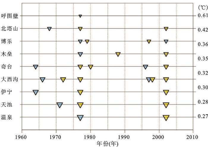
本文选取以新疆天山山脊为界的天山北部区域为研究区即北疆地区(包括有寒温带和温带两个气候带,其中寒温带气候带包括阿尔泰山气候区,温带气候带包括塔城气候区和布克赛尔气候区,额尔齐斯乌伦古气候区,准噶尔盆地气候区和天山北坡气候区[35])。本文使用的资料为1961~2010年北疆地区37个台站经过初步质量控制的逐日平均气温、最高气温、最低气温资料,同时使用北疆站点观察元数据(元数据指气象站点记录台站仪器更换、记录方法改变、台站迁移时间等信息)作为检验结果合理性和准确性的判断和序列订正的参考依据。本文以乌鲁木齐作为均一化研究的特例站点。在气温的均一化研究中选择了与乌鲁木齐相关性较强的9个站的作为参考站(图1)。
检查元数据记录发现,乌鲁木齐站在1961~2010年中有过2次迁站,分别为1975年12月31日由乌鲁木齐市西郊机场迁址到乌鲁木齐市南门幸福路(东侧),1999年12月31日由乌鲁木齐市南门幸福路 27 号迁址到乌鲁木齐市建国路 97 号。此外,还存在8次左右的仪器更换。
首先,利用PRODIGE方法[18]找到序列的多个断点。然后,可以得到年均最低气温(TN)的断点,计算方法为:
为了找到K,利用惩罚似然对数法[19]:
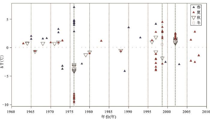
由(2)式就可以得到断点的集合。找出与每个待检站相关性最高的至少8个站点作为参考站,根据(1)可得到差值序列的断点。断点的检测是基于待检站与参考站进行对比在连续在两年内如果检测出3个或多个断点,则断点被认为有效。由于年均最低气温(TN)检测的断点比月时间序列和逐日时间序列要可靠,故先进行年均气温的检测。本文以乌鲁木齐站为例来说明PRODIGE方法的检测过程。乌鲁木齐站与相关性最高的9个参考站的差值序列(图2)及对比得到的断点总结(图3)。
由图2和图3可见,乌鲁木齐站至少有3个断点1976年、1999年和2002年。根据表1的元数据,检测出的断点的位置与乌鲁木齐站的迁站时间有比较好的对应,且2002年乌鲁木齐测量仪器发生变化。根据上面的分析,检测的断点比较准确,有利于后面进行进一步的检测。
图2 乌鲁木齐站与参考站的差值序列(|代表断点)
Fig.2 The differences between the annual minimum temperature sequences of Urumqi station and the reference station
图3 乌鲁木齐站断点检测(乌鲁木齐站与参考站的差值序列对比检测到的断点位置,从顶部到底部站点是按标准差的残差减小的顺序排列。从上到下,对比得到断点的可靠性增加)
Fig.3 The detected breakpoints for time series of the annual minmum temperature at Urumqi station
ACMANT(Adapted Caussinus Mestre Algorithm for Networks of Temperature series) [20]是新的均一化方法。它主要是根据PRODIGE方法在季节非均一性和周期上的修改,研究气温时间序列的季节非均一化的检测。ACMANT方法已经被COST ES0601(Advances in homogenisation methods of climate series: an integrated approach HOME )工作组证明能很好的使用于中高纬度地区的气温数据集的均一化。
ACMANT能准确对逐月时间序列的断点进行检测。ACMANT方法进行非均一性的时间的判断是通过拟合时间序列年平均值(TM)和相对范围内的季节性周期(TD)。
首先,应用PRODIGE方法对断点发生的年份进行比较准确的判定后;然后,再结合ACMANT方法,确定断点进行对比(图4)。从图4可知,乌鲁木齐最低气温断点发生在1976年、1999年和2002年。应用这一方法对月均最低气温/月均最高气温/年均最高气温/年均最低气温都做了检测,对得到的断点进行比较,发现所得到断点发生的位置比较接近。这为后续逐日最低气温、最高气温的均一化提供了关键的一步。
逐日气候数据序列的非均一性订正更多的是考虑了气候序列的平均态和中心趋势。而Della-Marta和Wanner[21]的HOM方法(Hight Order Moder method)则考虑了非均一性对气候极值的影响,实现了对逐日气候序列的均值和站点概率密度函数高阶矩的订正。
根据 HOMER(Homogenisation R language method)方法得到的北疆地区37个站点的断点的情况,再利用HOM方法(Hight Order Moder method)对这37个站点进行逐日最高气温和最低气温均一化。这种新的均一化逐日气温数据的方法,命名为HOMR-HOM。应用HOMR-HOM方法,建立1961~2010年北疆地区逐日最高气温和最低气温均一化的数据集。
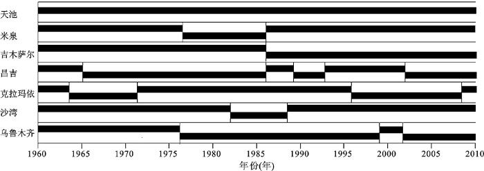
以乌鲁木齐站为例来描述逐日最低气温的订正过程。以上基于HOMER方法进行断点检测得到乌鲁木齐最低气温的断点发生1975年、1999年和2002年,断点情况与元数据迁移时期基本相符。同时,HOM方法要求待检站和参考站有比较高的相关性,在限制的时间段内,待检站和参考站都应该是均一的,称为均一区间 (HSPs)。乌鲁木齐站及参考站(昌吉、吉木萨尔、克拉玛依、米泉、沙湾、天池)的断点经过检测得到记录图(图5),基本与元数据站点迁移及仪器更改时期相符。
图5 乌鲁木齐站和参考站断点情况
Fig.5 The Urumqi station and the reference station of breakpoint
现在以乌鲁木齐站春季的均一化订正为例说明HOM方法订正的主要过程[21]:① 定义待检站的HSPs,选择一个相关性最好的参考站,使得参考站的HSP能够覆盖待检站的HSP1(均一区间1)和HSP2(均一区间2)。② 利用非线性模型对待检站的HSP1和参考站进行拟合,并使用参考站与待检站的非均一性后期的(HSP2)重合的数据来预测待检站的HSP2的气温,待检站(HSP2)的观测值与预测值产生差值序列。③ 拟合待检站HSP1和HSP2的概率分布,根据待检站的HSP1概率分布的十分位值,对差值序列进行区间划分。④ 利用平滑变化函数对区间差值进行拟合,来获得每个百分位的估计订正量;由待检站HSP2的概率分布,确定HSP2中每个观测值所在的百分位,对其进行订正;完成待检站的逐日气温的均一化。
HOM方法要求,参考站点与待检测站点之间必须有较高的相关性。在对待检测站的HSPs和参考站点进行非线性拟合时,从待检测站点最近的非均一性站点开始检测。必须使得参考序列的HSPs至少要涵盖非均一性前期3 a和非均一性后期3 a。但是在许多情况下,一个参考站也许只能适用于涵盖待检测站中的某一个HSPs,而不能适用于待检测站点所有的HSPs,这时对待检测站点进行均一化处理时,需要至少多于1个参考站点。
在2.1中HOMER检测已知,乌鲁木齐站在1976年、1999年、2002年存在断点,那么它就涵盖4段均一性区间HSP1(1961~1976),HSP2(1976~1999),HSP3(2000~2002),HSP4(2003~2010)。本节以乌鲁木齐站秋季逐日最低气温为例,选择4段均一性区间中的HSP1(1961~1976)为基准,分别选取涵盖断点1976年非均一性前期3 a和非均一性后期3 a的吉木萨尔、米泉、克拉玛依作为参考站。
1) 非线性模型拟合
使用非线性局部加权回归模型LOESS (nonliner locally weighted regression)[20]来对非均一前期待检测(yi)和参考站(xi)的逐日最低气温进行线性拟合。平滑模型为:
yi=g(xi)+
其中,g为回归函数,i是第i个观测值(i=1,2,…,Nmodel (观测值总个数)),
应用非线性模型(LOESS)模拟乌鲁木齐站和参考站吉木萨尔的最低气温在HSP1和HSP2(图略)。两条拟合线几乎都是线性的,但斜率显然都不为1。由于非均一性产生的方差的改变使得两条拟合曲线的斜率不同。对HSP1拟合的黑色曲线蓝色虚线的斜率都小于1,说明乌鲁木齐站的HSP1和HSP2逐日日最低气温的变化都小于吉木萨尔逐日日最低气温的变化。对于关于乌鲁木齐站点在HSP1和HSP2拟合曲线斜率的差异,可以发现乌鲁木齐在HSP1的逐日日最低气温微小于在HSP2的逐日气温方差,差别较小。
2) 百分位订正
根据乌鲁木齐站HSP1的累积概率分布将乌鲁木齐站HSP2观测值和模型拟合值之间的差值进行区间划分。HSP1和HSP2的累积概率分布(CDF)是L-moments[22]理论拟合,并使用分布拟合检验Kolmogorov-Smirnov test(K-S检验[40]) 对6种最优拟合分布的比较,对乌鲁木齐站的HSP1和HSP2的分布选用GEV分布。HSP2的分布已经得到,确定每个观测值所在的百分位(根据平滑变化的参数对区间十分位的差值拟合得到百分位的估计修订)进行修正。订正曲线呈现下降趋势,说明乌鲁木齐站HSP2的逐日最低气温变化应小于HSP1逐日最低气温变化值。对于所有的十分位差值的修正均值为+0.72°C。
将HSP1和基于HSP1修正的HSP2逐日最低气温变化看作新的HSP1,然后同样的方法,使 HSP3均一化到HSP1,最后将HSP4均一化到HSP1,这样得到乌鲁木齐站点秋季逐日最低气温的均一化值。HSP3、HSP4的非线性模拟、累计概率分布、百分位订正。将以上方法应用于其他3个季节,可以得到乌鲁木齐站长期逐日最低气温的数据。
针对得到了乌鲁木齐的逐日最低气温均一化序列,利用2.1的方法对乌鲁木齐站进行均一化验证。通过检验证明乌鲁木齐逐日最低气温为均一化序列。虽然,有少量不同的断点存在,但是这些断点是不可靠的。出现的原因可能在于参考站点存在断点。
以上分析表明,新的检测断点的方法HOMR-HOM是一种有效检测均一化的方法。应用HOMR-HOM,对北疆37个站点的逐日最高气温和最低气温进行了均一化处理,得到北疆站点基于HOMER-HOM一套完整的均一化数据,为后续研究北疆地区气温的极值变换奠定了良好的基础。
经计算得到37个站50 a年平均最低气温订正前为-0.22°C,订正后为 -0.20°C,年平均最高气温订正前为12.6°C,订正后为12.34°C。图6a,图6b分别为订正后的年平均最低/最高气温与订正前的年平均最低/最高气温的差值分布,可以看出订正幅度基本在 -0.8~+0.8°C之间,订正后北疆地区最低气温大多数台站较订正前气温变高;订正后北疆地区最高气温大多数台站较订正前气温变低。
图6 原序列年平均最低气温与订正后的年平均最低气温的差值(°C) (a);原序列年平均最高气温与订正后的年平均最高气温的差值(°C) (b)
Fig.6 Difference (°C) between original sequence of annual mean minimum temperature and the revised annual average minimum temperature(a), difference (°C) between original sequence of annual mean maximum temperature and the revised annual average maximum temperature(b)
北疆地区实际研究中应用的数据存在一定的问题,但这些问题是不可避免的。如何来减少人为因素造成的误差,如:站点迁移、观察方法改变、观察仪器的变更等等,这些存在的问题。国内外部分学者意识到,这些误差足以改变气候变化研究的结果。北疆是生态环境较为敏感的区域,一直以来认为是逐年暖湿化的改变,这些结论有些已经上升到国家战略。如果研究成果,在基础数据中存在问题,得到相反的结论会造成的严重的后果。因此,进行均一化研究的十分有必要。虽然技术不是太成熟,随着时间的推移,高质量数据作用的显现会越来越重要。通过,本文研究得到以下结论:
1) 新组合均一化逐日气温的方法-HOMR-HOM方法,通过案例分析,可以较好的检测断点和订正数据。通过订正后北疆地区大多数台站较订正前气温存在一定的差异,这说明观察数据存在一定的问题。均一化后的数据集的使用,会逐渐和以往观察数据得出结论做比较,来确定数据集能否直接用来进行极端气候事件研究。
2) 以乌鲁木齐为例的研究表明,新的均一化方法可以很好的应用到北疆地区的逐日气候均一化研究。但是,该方法不能只能在中高纬度地区进行研究,具有一定的局限性。
3) 应用该方法对逐日最高气温和最低气温进行了均一化订正,得到北疆地区逐日最高气温和最低气温数据集。研究发现北疆地区观测最高气温数据比均一化后数据高,观测最低气温数据比均一化后数据低。
4) 得到的均一化数据集为未来北疆地区极端气候变化研究打下了良好的数据基础。均一化数据集,可以减少人为因素对气候变化研究影响,具有重要的研究价值。
The authors have declared that no competing interests exist.
| [1] |
Recent Changes in Climate Extremes in the Caribbean Region [J].https://doi.org/10.1029/2002JD002251 URL [本文引用: 1] 摘要
[1] A January 2001 workshop held in Kingston, Jamaica, brought together scientists and data from around the Caribbean region and made analysis of indices of extremes derived from daily weather observation in the region possible. The results of the analyses indicate that the percent of days having very warm maximum or minimum temperatures increased strongly since the late 1950s while the percent of days with very cold temperatures decreased. One measure of extreme precipitation shows an increase over this time period while the one analyzed measure of dry conditions, the maximum number of consecutive dry days, is decreasing. These changes generally agree with what is observed in many other parts of the world.
|
| [2] |
Effects of Changing Exposure of Thermometers at Land Stations [J].https://doi.org/10.1002/joc.3370140102 URL [本文引用: 1] 摘要
Abstract In view of the implications for the assessment of climatic changes since the mid-nineteenth century, systematic changes of exposure of thermometers at land stations are reviewed. Particular emphasis is laid on changes of exposure during the late nineteenth and early twentieth century when shelters often differed considerably from the Stevenson screens, and variants thereof, which have been prevalent during the past few decades. It is concluded that little overall bias in land surface air temperature has accumulated since the late nineteenth century: however, the earliest extratropical data may have been biased typically 0.2掳C warm in summer and by day, and similarly cold in winter and by night, relative to modern observations. Furthermore, there is likely to have been a warm bias in the tropics in the early twentieth century: this bias, implied by comparisons between Stevenson screens and the tropical sheds then in use, is confirmed by comparisons between coastal land surface air temperatures and nearby marine surface temperatures, and was probably of the order of 0.2掳C.
|
| [3] |
The Effect of Radiation Screens on Nordic Time Series of Mean Temperature [J].https://doi.org/10.1002/(SICI)1097-0088(199712)17:15<1667::AID-JOC221>3.0.CO;2-D URL [本文引用: 2] 摘要
Abstract A short survey of the historical development of temperature radiation screens is given based upon research in the archives of the Nordic meteorological institutes. In the middle of the nineteenth century most thermometer stands were open shelters, free-standing or fastened to a window or wall. Most of these were soon replaced by wall or window screens, i.e. small wooden or metal cages. Large free-standing screens were also introduced in the nineteenth century, but it took to the 1980s before they had replaced the wall screens completely in all Nordic countries. During recent years, small cylindrical screens suitable for automatic weather stations have been introduced. At some stations they have replaced the ordinary free-standing screen as part of a gradual move towards automation. The first free-standing screens used in the Nordic countries were single louvred. They were later improved by double louvres. Compared with observations from ventilated thermometers the monthly mean temperatures in the single louvred screens were 0·2–0·4°C higher during May–August, whereas in the double louvred screens the temperatures were unbiased. Unless the series are adjusted, this improvement may lead to inhomogeneities in long climatic time series. The change from wall screen to free-standing screen also involved a relocation from the microclimatic influence of a house to a location free from obstacles. Tests to evaluate the effect of relocation by parallel measurements yielded variable results. However, the bulk of the tests showed no effect of the relocation in winter, whereas in summer the wall screen tended to be slightly warmer (0·0–0·3°C) than the double louvred screen. At two Norwegian sites situated on steep valley slopes, the wall screen was ca . 0·5°C colder in midwinter. The free-standing Swedish shelter, which was used at some stations up to 1960, seems to have been overheated in spring and summer (maximum overheating of about 0·4°C in early summer). The new screen for automatic sensors appears to be unbiased compared with the ordinary free-standing screen concerning monthly mean temperature. 08 1997 Royal Meteorological Society.
|
| [4] |
Probabilistic estimates of future changes in California temperature and precipitation using statistical and dynamical downscaling [J].https://doi.org/10.1007/s00382-012-1337-9 URL [本文引用: 1] 摘要
Sixteen global general circulation models were used to develop probabilistic projections of temperature (T) and precipitation (P) changes over California by the 2060s. The global models were downscaled with two statistical techniques and three nested dynamical regional climate models, although not all global models were downscaled with all techniques. Both monthly and daily timescale changes in T and P are addressed, the latter being important for a range of applications in energy use, water management, and agriculture. The T changes tend to agree more across downscaling techniques than the P changes. Year-to-year natural internal climate variability is roughly of similar magnitude to the projected T changes. In the monthly average, July temperatures shift enough that that the hottest July found in any simulation over the historical period becomes a modestly cool July in the future period. Januarys as cold as any found in the historical period are still found in the 2060s, but the median and maximum monthly average temperatures increase notably. Annual and seasonal P changes are small compared to interannual or intermodel variability. However, the annual change is composed of seasonally varying changes that are themselves much larger, but tend to cancel in the annual mean. Winters show modestly wetter conditions in the North of the state, while spring and autumn show less precipitation. The dynamical downscaling techniques project increasing precipitation in the Southeastern part of the state, which is influenced by the North American monsoon, a feature that is not captured by the statistical downscaling.
|
| [5] |
Errors in Early Temperature Series Arising from Changes in Style of Measuring Time, Sampling Schedule and Number of Observations [J].https://doi.org/10.1023/A:1014962623762 URL [本文引用: 1] 摘要
Study of the Padova series (1725鈥搕oday) is a useful example, of general interest, of a critical revision of long time series. These are composed of a number of inhomogeneous parts, each of them with mean daily values, and extremes, computed in different ways, based on observations taken at different times, or with the time expressed in different styles. Imprecise clocks, little care for the schedule established for meteorological readings, changing style of evaluating time, inappropriate choice of observing schedules, too small a number of readings to compute the daily average, generated errors that caused significant departures in time series, that could be interpreted as a climate signal. In the past, average values were obtained with only a few daily measurements. The first problem is to correct the data and extrapolate the hourly temperatures needed to evaluate the daily minimum, maximum and average values in a homogeneous way. The change of style in temporal reference introduced spurious seasonal changes. Styles (or combinations of styles) used were: Italian time in use till 1789, in which the hours were computed starting from twilight; apparent solar time based on the actual motion of the sun; mean solar time based on the average motion of the sun; local time referred to the actual passage of the sun across the local meridian (local culmination); French time starting at midnight and regulated on the local culmination; Western European Time regulated on the culmination of fictitious average solar motion on a reference meridian 15掳 East. A test was performed to verify whether the times chosen for readings were appropriate, in particular when observations were performed not close to the daily minimum and maximum. In effect, in the early period with Morgagni and Toaldo, the choice of schedule of observations was good, but afterwards the introduction of new observations, not always established at the most appropriate schedule, reduced the representativity of the data. The error in calculating the daily average temperature after a given number of observations taken at different hours of the day has been analysed. National, and especially international recommendations have been particularly important in the choice of observations times, and in determining averages. These recommendations have been simultaneously applied on a large number of sites, causing an in-homogeneity that may be misinterpreted as a well-documented, widespread climate change.
|
| [6] |
Effects of Changes in Algorithms Used for the Calculation of Australian Mean Temperature [J].https://doi.org/10.1016/j.atmosenv.2003.11.036 URL [本文引用: 1] 摘要
temperature
|
| [7] |
点观测气象序列的非均一性研究 [J]. |
| [8] |
A homogeneity test applied to precipitation data [J].https://doi.org/10.1002/joc.3370060607 URL [本文引用: 1] 摘要
Abstract In climate research it is important to have access to reliable data which are free from artificial trends or changes. One way of checking the reliability of a climate series is to compare it with surrounding stations. This is the idea behind all tests of the relative homogeneity. Here we will present a simple homogeneity test and apply it to a precipitation data set from south-western Sweden. More precisely we will apply it to ratios between station values and some reference values. The reference value is a form of a mean value from surrounding stations. It is found valuable to include short and incomplete series in the reference value. The test can be used as an instrument for quality control as far as the mean level of, for instance, precipitation is concerned. In practice it should be used along with the available station history. Several non-homogeneities are present in these series and probably reflect a serious source of uncertainty in studies of climatic trends and climatic change all over the world. The significant breaks varied from 5 to 25 per cent for this data set. An example illustrates the importance of using relevant climatic normals that refer to the present measurement conditions in constructing maps of anomalies.
|
| [9] |
Sajecki P J F. Testing for Homogeneity in Temperature Time Series at Canadian Climate Stations [J]. |
| [10] |
A New Method for Detecting Undocumented Discontinuities in Climatological Time Series [J].https://doi.org/10.1002/joc.3370150403 URL [本文引用: 1] 摘要
Abstract The development of homogeneous climatological time series is a crucial step in examining climate fluctuations and change. We review and test methods that have been proposed previously for detecting inhomogeneities, and introduce a new method we have developed. This method is based on a combination of regression analysis and non-parametric statistics. After evaluation against other techniques, using both simulated and observed data, our technique appears to have the best overall performance.
|
| [11] |
Bayesian change-point analysis in hydrometeorological time series [J]. |
| [12] |
A technique for the identification of inhomogeneities in Canadian temperature series [J]. |
| [13] |
Homogenization of daily temperatures over Canada [J]. |
| [14] |
|
| [15] |
Multiple Analysis of Series for Homogenization (MASHv3.03). Hungarian Meteorological Service H-1525, P.O. Box 38, Budapest,
|
| [16] |
The manual of Multiple Analysis of Series for Homogenization (MASH). Hungarian Meteorological Service, Budapest, Hungary. 2008. [Available from ]. |
| [17] |
Application of multiple analysis of series for homogenization (MASH) to Beijing daily temperature series 1960-2006 [J].https://doi.org/0.1007/s00376-009-9052-0 Magsci [本文引用: 1] 摘要
Homogenization of climate observations remains a challenge to climatechange researchers, especially in cases where metadata (e.g., probable dates ofbreak points) are not always available. To examine the influence of metadata onhomogenizing climate data, the authors applied the recently developed MultipleAnalysis of Series for Homogenization (MASH) method to the Beijing (BJ) dailytemperature series for 1960--2006 in three cases with different references: (1)13M---considering metadata at BJ and 12 nearby stations; (2)13NOM---considering the same 13 stations without metadata; and (3)21NOM---considering 20 further stations and BJ without metadata. The estimatedmean annual, seasonal, and monthly inhomogeneities are similar between the 13Mand 13NOM cases, while those in the 21NOM case are slightly different. Thedetected biases in the BJ series corresponding to the documented relocationdates are as low as -0.71<sup>o</sup>C, -0.79<sup>o</sup>C, and -0.5<sup>o</sup>Cfor the annual mean in the 3 cases, respectively. Otherbiases, including those undocumented in metadata, are minor. The resultssuggest that any major inhomogeneity could be detected via MASH, albeit withminor differences in estimating inhomogeneities based on the differentreferences. The adjusted annual series showed a warming trend of 0.337, 0.316,and 0.365<sup>o</sup>C (10 yr)<sup>-1</sup> for the three cases, respectively, smallerthan the estimate of 0.453<sup>o</sup>C (10 yr)<sup>-1</sup> in the original series,mainly due to the relocation-induced biases. The impact of the MASH-typehomogenization on estimates of climate extremes in the daily temperature seriesis also discussed.
|
| [18] |
Choosing a linear model with a random number of change-points and outliers [J].https://doi.org/10.1023/A:1003230713770 URL [本文引用: 1] 摘要
The problem of determining a normal linear model with possible perturbations, viz. change-points and outliers, is formulated as a problem of testing multiple hypotheses, and a Bayes invariant optimal multi-decision procedure is provided for detecting at most k (k > 1) such perturbations. The asymptotic form of the procedure is a penalized log-likelihood procedure which does not depend on the loss function nor on the prior distribution of the shifts under fairly mild assumptions. The term which penalizes too large a number of changes (or outliers) arises mainly from realistic assumptions about their occurrence. It is different from the term which appears in Akaike‘s or Schwarz‘ criteria, although it is of the same order as the latter. Some concrete numerical examples are analyzed.
|
| [19] |
Newest developments of ACMANT [J].https://doi.org/10.5194/asr-6-7-2011 URL [本文引用: 1] 摘要
The seasonal cycle of radiation intensity often causes a marked seasonal cycle in the inhomogeneities (IHs) of observed temperature time series, since a substantial portion of them have direct or indirect connection to radiation changes in the micro-environment of the thermometer. Therefore the magnitudes of temperature IHs tend to be larger in summer than in winter. A new homogenisation method, the Adapted Caussinus 鈥 Mestre Algorithm for Networks of Temperature series (ACMANT) has recently been developed which treats appropriately the seasonal changes of IH-sizes in temperature time series. The performance of ACMANT was proved to be among the best methods (together with PRODIGE and MASH) in the efficiency test procedure of COST ES0601 project. A further improved version of the ACMANT is described in this paper. In the new version the ANOVA procedure is applied for correcting inhomogeneities, and with this change the iterations applied in the earlier version have become unnecessary. Some other modifications have also been made, from which the most important one is the new way for estimating the timings of IHs. With these modifications the efficiency of the ACMANT has become even higher, therefore its use is strongly recommended when networks of monthly temperature series from mid- or high geographical latitudes are subjected to homogenisation. The paper presents the main properties and the operation of the new ACMANT.
|
| [20] |
Locally-weighted fitting: An approach to fitting analysis by local fitting [J]. |
| [21] |
A method of homogenizing the extremes and mean of daily temperature measurements [J]. |
| [22] |
L-Moments: Analysis and Estimation of Distributions Using Linear Combinations of Order Statistics [J]. |

/
| 〈 |
|
〉 |


